Excel Lookup And Reference Functions: A Step By Step Guide

Excel lookup and reference functions are powerful tools for finding and retrieving data from spreadsheets, enabling efficient data analysis and management. These functions allow users to search for specific values, match data across tables, and reference cells dynamically, streamlining workflows. 

Key functions include VLOOKUP and HLOOKUP, which search vertically or horizontally for a value in a table and return a corresponding value from another column or row. INDEX and MATCH offer more flexibility, combining to pinpoint data by row and column indices, often outperforming VLOOKUP in complex scenarios. 

XLOOKUP, introduced in newer Excel versions, enhances lookup capabilities with simpler syntax and support for approximate or exact matches. Other functions like OFFSET, INDIRECT, and CHOOSE facilitate dynamic referencing and data manipulation. 

What Are Excel Lookup And Reference Functions? 

Excel lookup and reference functions are tools designed to search, retrieve, and reference data within spreadsheets, simplifying data management and analysis. These functions enable users to locate specific values, match data across ranges, and dynamically reference cells.

Different Lookup Functions In Excel 

Excel’s lookup functions are essential tools for searching, retrieving, and manipulating data within spreadsheets, enabling users to efficiently manage large datasets, automate tasks, and create dynamic reports. These functions allow users to locate specific values in a range or table and return corresponding data from another column or row. 

Excel provides several lookup functions, each with unique features suited to different scenarios. The most prominent lookup functions are VLOOKUP, HLOOKUP, XLOOKUP, and the combination of INDEX and MATCH.  

1. VlookUp 

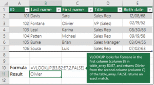
VLOOKUP is one of Excel’s most widely used lookup functions, designed to search for a value in the first column of a table and return a corresponding value from a specified column in the same row. Excel Lookup And Reference Functions are essential for your record keeping. 

• lookup_value: The value to search for in the first column of the table.
• table_array: The range containing the data, with the lookup column as the first column.
• col_index_num: The column number (relative to the table_array) from which to return a value.
• range_lookup: Optional; TRUE comes for approximate match (requires sorted data) or FALSE for exact match.  

Example:- 

Source( support.microsoft.com) 

How It Works

VLOOKUP searches vertically down the first column of the specified table_array for the lookup_value. Once found, it retrieves the value from the same row in the column specified by col_index_num. If range_lookup is TRUE (or omitted), it performs an approximate match, assuming the first column is sorted in ascending order. If FALSE, it requires an exact match.

Advantages

• Simple to use for straightforward vertical lookups.
• Widely supported across all Excel versions.
• Useful for tasks like retrieving prices, names, or other data associated with a key value.

Limitations

• Only searches in the first column of the table_array.
• Cannot look to the left of the lookup column.
• Performance may slow with very large datasets.
• Requires exact column indexing, which can break if columns are reordered.

Use Case

VLOOKUP is ideal for scenarios like inventory management, where you need to retrieve product details based on a unique identifier, such as a SKU or product code. Excel lookup and reference functions are crucial for your record keeping. 

2. Hlookup 

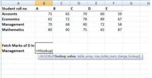
HLOOKUP is the horizontal counterpart to VLOOKUP, designed for datasets where the lookup values are in the first row of a table, and the return values are in a specified row below.

• lookup_value: The value to search for in the first row of the table.
• table_array: The range containing the data, with the lookup row as the first row.
• row_index_num: The row number (relative to the table_array) from which to return a value.
• range_lookup: Optional; TRUE comes for approximate match (sorted data) or FALSE for exact match.  

How It Works

HLOOKUP searches horizontally across the first row of the table_array for the lookup_value and retrieves the value from the specified row in the same column. Like VLOOKUP, it helps in exact (FALSE) or near about (TRUE) matches.   

Example:   

Source( support.microsoft.com) 

Advantages

• It is applicable for horizontally organized data, such as timelines or category-based tables.
• Simple syntax, similar to VLOOKUP.

Limitations

• Limited to searching the first row only.
• Cannot retrieve data above the lookup row.
• Less commonly used due to the prevalence of vertically structured data.

Use Case

HLOOKUP is suitable for datasets like monthly reports or dashboards where data is organized by time periods across columns. This Excel lookup and reference functions are essential for your accurate record keeping. 

3. Xlookup 

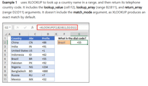
Introduced in Excel 365 and Excel 2019 (later versions), XLOOKUP is a modern, effective lookup function that make over  many limitations of VLOOKUP and HLOOKUP.  

• lookup_value: The value to search for.
• lookup_array: The range or array to search in.
• return_array: The range or array from which to return a value.
• if_not_found: Optional; value to return if no match is found (e.g., “Not Found”).
• match_mode: Optional; 0 (exact), 1 (exact or next larger), -1 (exact or next smaller), or 2 (wildcard match).
• search_mode: Optional; 1 (first-to-last), -1 (last-to-first), or binary search options.

How It Works

XLOOKUP searches the lookup_array for the lookup_value and returns the corresponding value from the return_array. It supports bidirectional searches (vertical or horizontal), exact or approximate matches, and reverse-order searches. The if_not_found parameter eliminates the need for error-handling functions like IFERROR. 

Example:  

Source(Support.microsoft.com) 

Advantages

• Searches in any direction (left, right, up, or down).
• Handles errors gracefully with the if_not_found parameter.
• Supports wildcard matches and reverse searches.
• More intuitive syntax than VLOOKUP/HLOOKUP.

Limitations

• Not available in older Excel versions (pre-2019).
• Slightly more complex for beginners due to additional parameters.

Use Case

XLOOKUP is ideal for complex datasets requiring flexible lookups, such as financial models or cross-referenced tables, where data may not be structured for VLOOKUP/HLOOKUP.

4. Index And Match 

The combination of INDEX and MATCH provides a powerful, flexible alternative to VLOOKUP and HLOOKUP, often used for advanced lookups.

Syntax

• INDEX: =INDEX(array, row_num, [column_num])
  • Returns a value at the intersection of a specified row and column in a range.
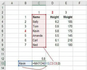
• MATCH: =MATCH(lookup_value, lookup_array, [match_type])
  • Give away the relative position of a value in a range (0 for exact, 1 for next smaller, -1 for next larger).
• Combined: =INDEX(return_range, MATCH(lookup_value, lookup_array, 0))

How It Works

MATCH finds the position of the lookup_value in the lookup_array, and INDEX uses that position to retrieve a value from the return_range. This combination allows lookups in any direction and is more dynamic than VLOOKUP.   

Example:-  

Source( corporate finance institute.com) 

 Source( corporate Finance institute.com) 

Advantages

• Can look left or right of the lookup column.
• More flexible and robust than VLOOKUP/HLOOKUP.
• Works with unsorted data for exact matches.

Limitations

• Requires two functions, making it slightly more complex.
• May be slower in very large datasets compared to XLOOKUP.

Use Case

INDEX and MATCH are perfect for scenarios requiring lookups in non-standard table layouts or when columns may be reordered, such as in dynamic dashboards or data analysis.

Different Reference Functions In Excel 

Excel’s reference functions are powerful tools that allow users to dynamically locate and retrieve data from specific cells or ranges within a spreadsheet. These functions are essential for creating flexible, automated, and dynamic worksheets, especially when working with large datasets or complex models. 

Unlike lookup functions (e.g., VLOOKUP, XLOOKUP), which primarily search for values, reference functions focus on navigating and manipulating cell references or ranges based on specific criteria. 

Below is a detailed explanation of the key reference functions in Excel—INDEX, OFFSET, INDIRECT, CHOOSE, ADDRESS, and ROW/COLUMN—including their syntax, functionality, use cases, and examples, all within a 1000-word limit.

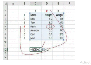
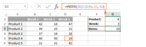
1. INDEX 

The INDEX function retrieves a value or range from a specified position within a given array or range.

• array: The range or array from which to return a value.
• row_num: The row position in the array (required).
• column_num: The column position in the array (optional; used for multi-column ranges).

How It Works  

INDEX returns the value at the intersection of the specified row and column in the array. If used with a single-column or single-row range, only row_num or column_num is needed. INDEX is often paired with MATCH for dynamic lookups but is a reference function at its core. 

Example:- 

Source(ablebits.com) 

Use Case

INDEX is ideal for retrieving specific values from a table or creating dynamic ranges for charts or calculations.

Advantages

• Flexible for single-cell or range references.
• Can be combined with MATCH for advanced lookups.
• Works with both rows and columns.

Limitations

• Requires precise row/column numbers, which can be cumbersome without MATCH.
• Less intuitive for beginners compared to lookup functions.

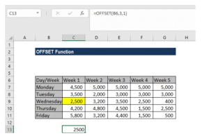
2. OFFSET 

The OFFSET function returns a range that is offset from a starting cell by a specified number of rows and columns. 

• reference: The starting cell or range.
• rows: Number of rows to move (positive = down, negative = up).
• cols: Number of columns to move (positive = right, negative = left).
• height: Optional; number of rows in the returned range.
• width: Optional; number of columns in the returned range.  

How It Works

OFFSET starts at the reference cell and moves by the specified rows and cols to return a new range or single cell. The height and width parameters define the size of the returned range.  

Example:- 

Source(Corporatefinanceinstitute.com) 

Use Case

OFFSET is useful for creating dynamic ranges in charts, dropdown lists, or calculations that adjust based on user input or data changes.

Advantages

• Creates dynamic ranges that adapt to data changes.
• Useful for dashboards and reports requiring flexible references.

Limitations

• Volatile function (recalculates with every worksheet change, potentially slowing performance).
• Can be complex to debug if misused.

3. INDIRECT 

The INDIRECT function returns a reference specified by a text string, allowing dynamic cell or range referencing.  

• ref_text: A text string representing a cell reference (e.g., “A1” or “Sheet2!B5”).
• a1: Optional; TRUE for A1-style references (default), FALSE for R1C1-style. 

How It Works

INDIRECT converts a text string into a valid cell or range reference, enabling dynamic referencing based on formulas or user input. It’s particularly useful for referencing different sheets or ranges dynamically. 

Example:-   

Source( https://www.ablebits.com/)

Use Case

INDIRECT is ideal for creating formulas that reference different sheets or ranges based on dropdown selections or text inputs, such as in multi-sheet reports.

Advantages

• Enables dynamic referencing without hardcoding cell addresses.
• Useful for cross-sheet operations or template-driven models.

Limitations

• Volatile, like OFFSET, which can impact performance.
• Error-prone if ref_text is invalid or misspelled.

4. CHOOSE 

The CHOOSE function returns a value from a list based on a specified index number.

• index_num: The position (1, 2, 3, etc.) of the value to return.
• value1, value2, …: The list of values or references to choose from (up to 254).

Example:-  

Source(ablebits.com) 

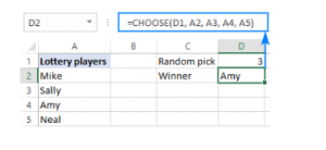
How It Works

CHOOSE selects a value or reference from the provided list based on the index_num. The index must be a number between 1 and the number of values provided.

Use Case

CHOOSE is useful for creating simple dropdown-driven calculations or selecting specific ranges/values based on user input, such as in scenario analysis.

Advantages

• Simple and intuitive for selecting from a predefined list.
• Can return values or cell references.

Limitations

• Limited to 254 values.
• Less flexible than INDEX or OFFSET for large datasets.

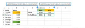
5. ADDRESS 

The ADDRESS function creates a cell reference as a text string based on specified row and column numbers. 

• row_num: The row number for the reference.
• column_num: The column number (e.g., 1 for A, 2 for B).
• abs_num: Optional; 1 (absolute, e.g., $A$1), 2 (row absolute, e.g., A$1), 3 (column absolute, e.g., $A1), 4 (relative, e.g., A1).
• a1: Optional; TRUE for A1-style (default), FALSE for R1C1-style.
• sheet_text: Optional; the worksheet name for the reference.

How It Works

ADDRESS generates a text string representing a cell address, which can be used with INDIRECT for dynamic referencing.  

Example:- 

Source(Ablebits.com) 

Use Case

ADDRESS is useful for generating dynamic cell references in formulas, especially when combined with INDIRECT for automated reporting.

Advantages

• Creates flexible, formula-driven cell references.
• Useful in complex models requiring programmatically generated addresses.

Limitations

• Returns text, so it often requires INDIRECT to be functional.
• Can be complex for beginners.

Excel Lookup & Reference Formulas 

Below is a concise list of Excel’s primary lookup functions, including their formulas (syntax) and a brief description of their purpose. These functions are designed to search for and retrieve data from specific ranges or tables in a spreadsheet.  

1. VLOOKUP (Vertical Lookup)

• Formula: =VLOOKUP(lookup_value, table_array, col_index_num, [range_lookup])
• Purpose: Searches for a value in the first column of a table and returns a value from a specified column in the same row.
• Parameters:
  • lookup_value: Value to search for.
  • table_array: Range containing the data (lookup value in first column).
  • col_index_num: Column number to return a value from.
  • range_lookup: TRUE (approximate match, sorted data) or FALSE (exact match).

2. HLOOKUP (Horizontal Lookup)

• Formula: =HLOOKUP(lookup_value, table_array, row_index_num, [range_lookup])
• Purpose: Searches for a value in the first row of a table and returns a value from a specified row in the same column.
• Parameters:
  • lookup_value: Value to search for.
  • table_array: Range with lookup value in first row.
  • row_index_num: Row number to return a value from.
  • range_lookup: TRUE (approximate) or FALSE (exact).

3. XLOOKUP (Advanced Lookup)

• Formula: =XLOOKUP(lookup_value, lookup_array, return_array, [if_not_found], [match_mode], [search_mode])
• Purpose: Searches a range for a value and returns a corresponding value from another range, with flexible search options.
• Parameters:
  • lookup_value: Value to search for.
  • lookup_array: Range to search in.
  • return_array: Range to return a value from.
  • if_not_found: Value if no match (optional).
  • match_mode: 0 (exact), 1 (next larger), -1 (next smaller), 2 (wildcard).
  • search_mode: 1 (first-to-last), -1 (last-to-first), or binary search.

4. INDEX and MATCH (Combined Lookup)

• Formulas:
  • INDEX: =INDEX(array, row_num, [column_num])
  • MATCH: =MATCH(lookup_value, lookup_array, [match_type])
  • Combined: =INDEX(return_range, MATCH(lookup_value, lookup_array, 0))
• Purpose: INDEX returns a value at a specified position; MATCH finds the position of a value. Together, they enable flexible lookups.
• Parameters:
  • INDEX:
    • array: Range to retrieve from.
    • row_num: Row position.
    • column_num: Column position (optional).
  • MATCH:
    • lookup_value: Value to search for.
    • lookup_array: Range to search in.
    • match_type: 0 (exact), 1 (next smaller), -1 (next larger).

All The Reference Functions Formulas 

Below is a concise list of Excel’s primary reference functions, including their formulas (syntax) and a brief description of their purpose. These functions are designed to dynamically locate, manipulate, or create cell references and ranges in a spreadsheet, enabling flexible data navigation and automation. 

1. INDEX

• Formula: =INDEX(array, row_num, [column_num])
• Purpose: Returns a value or range at the intersection of a specified row and column in a given array.
• Parameters:
  • array: The range or array to retrieve from.
  • row_num: The row position in the array.
  • column_num: The column position (optional for single-column ranges).

2. OFFSET

• Formula: =OFFSET(reference, rows, cols, [height], [width])
• Purpose: Returns a range offset from a starting cell by a specified number of rows and columns.
• Parameters:
  • reference: The starting cell or range.
  • rows: Number of rows to move (positive = down, negative = up).
  • cols: Number of columns to move (positive = right, negative = left).
  • height: Number of rows in the returned range (optional).
  • width: Number of columns in the returned range (optional).

3. INDIRECT

• Formula: =INDIRECT(ref_text, [a1])
• Purpose: Returns a reference specified by a text string, enabling dynamic cell or range referencing.
• Parameters:
  • ref_text: A text string representing a cell reference (e.g., “A1” or “Sheet2!B5”).
  • a1: TRUE for A1-style references (default) or FALSE for R1C1-style (optional).

4. CHOOSE

• Formula: =CHOOSE(index_num, value1, [value2], …)
• Purpose: Returns a value or reference from a list based on a specified index number.
• Parameters:
  • index_num: The position (1, 2, 3, etc.) of the value to return.
  • value1, value2, …: The list of values or references (up to 254).

5. ADDRESS

• Formula: =ADDRESS(row_num, column_num, [abs_num], [a1], [sheet_text])
• Purpose: Creates a text string for a cell reference based on specified row and column numbers.
• Parameters:
  • row_num: The row number for the reference.
  • column_num: The column number (e.g., 1 for A, 2 for B).
  • abs_num: 1 (absolute, e.g., $A$1), 2 (row absolute, e.g., A$1), 3 (column absolute, e.g., $A1), 4 (relative, e.g., A1) (optional).
  • a1: TRUE for A1-style (default) or FALSE for R1C1-style (optional).
  • sheet_text: Worksheet name for the reference (optional).

6. ROW

• Formula: =ROW([reference])
• Purpose: Returns the row number of a specified cell or the current cell if no reference is provided.
• Parameters:
  • reference: The cell or range to evaluate (optional; defaults to the cell containing the formula).

7. COLUMN

• Formula: =COLUMN([reference])
• Purpose: Returns the column number of a specified cell or the current cell if no reference is provided.
• Parameters:
  • reference: The cell or range to evaluate (optional; defaults to the cell containing the formula).

Vlookup Excel Functions Arguments   

The VLOOKUP function in Excel is a widely used lookup function that searches for a value in the first column of a table and returns a corresponding value from a specified column in the same row. Below is a detailed explanation of the VLOOKUP function’s arguments, including their purpose, usage, and considerations.

Arguments Of VLOOKUP

1. Lookup_Value 

Purpose: The value to search for in the first column of the table_array.

Description: This can be a specific value (e.g., a number, text, or cell reference) or a formula that evaluates to a value. The lookup_value is compared against the first column of the table_array.

Considerations:

• The lookup_value must exist in the first column of the table_array for an exact match (if range_lookup is FALSE).
• Text values are case-insensitive (e.g., “apple” matches “Apple”).
• If the lookup_value is not found and range_lookup is TRUE, it requires the first column to be sorted in ascending order for an approximate match.

2. Table_Array 

Purpose: The range or table where the data is located, with the lookup column as the first column.

Description: This is the range of cells containing the data to search and retrieve from. The first column of this range is where VLOOKUP searches for the lookup_value, and the return value comes from another column in the same row.

Considerations:

• The first column must contain the lookup_value for successful matches.
• Use absolute references (e.g., $A$2:$C$10) to prevent range shifts when copying the formula.
• The table_array can span multiple columns but must include the lookup and return columns.

3. Col_Index_num 

Purpose: The column number in the table_array from which to return a value.

Description: This specifies which column in the table_array contains the value to return, relative to the first column (which is 1). For example, if table_array is A2:C10, column A is 1, B is 2, and C is 3.

Considerations:

• The col_index_num must be a positive integer and not exceed the number of columns in the table_array.
• If columns are added or removed in the table_array, the col_index_num may need adjustment, as it’s not dynamic.
• Errors occur if col_index_num is invalid (e.g., 0 or greater than the table_array’s column count).

 4. Range_lookup 

Purpose: Specifies whether to perform an exact or approximate match.

Description:

• TRUE (or omitted): Performs an approximate match, assuming the first column of table_array is sorted in ascending order. VLOOKUP returns the closest match less than or equal to the lookup_value.
• FALSE: Requires an exact match. If the lookup_value is not found, VLOOKUP returns an #N/A error.

Considerations:

• For approximate matches (TRUE), the first column must be sorted in ascending order to avoid incorrect results.
• Use FALSE for unique identifiers (e.g., product codes, IDs) to ensure precision.
• Omitting range_lookup defaults to TRUE, which may lead to unexpected results if the data isn’t sorted.

Final Takeaway 

Hence, these are some of the crucial facts about Excel Lookup and reference functions can be easier for you to understand once you read this article. Additionally this can boost your brand value to a greater level. 

You can share your views and opinions in our comment box. This will boost the chances of delivering better content next time with ease. Share your views on it within a limited time. 

• Author
• Recent Posts

ICA Edu Skills Team

Working with businesses in diverse industries. I'm passionate about helping others understand and manage their finances effectively. This blog is where I share practical tips, insightful guides, and the latest updates on accounting, taxation, GST, TallyPrime, and advanced Excel. Feel free to ask questions, leave comments.

Latest posts by ICA Edu Skills Team (see all)

• Excel Lookup And Reference Functions: A Step By Step Guide - October 31, 2025
• How To Create A Database Design In Excel: Step By Step Guide - October 24, 2025
• How To Use Mail Merge In Word - October 17, 2025