.jpg)


15+ Advanced Excel Formulas: Learn to Become an Excel Pro
Do you have any idea about 15+ Advanced Excel Formulas? But for sure you have used some of these basic functions like SUMIF, IF OR, COUNT, and many more. These are the basic general Excel functions that we mostly use while working with large data on Excel Sheets.
But most of us have never used advanced Excel functions and formulas. No need to worry about this. We are here with a complete guide of updated and advanced Excel formulas that add value to your skills and knowledge.
Today, most industries need experts with advanced skills in Microsoft Excel. To manage their strong database for running a successful business.
So, we are here to help you in upgrading your Excel skills with our comprehensive guide on advanced Excel Formulas. Even it will help you to grab new job opportunities.
Any doubt if remain then you can join our advanced excel course.
Table of Contents
1.VLOOKUP()Function
Scenario:
Are you running a cloth shop? If yes then most probably sometimes you are puzzled by inventory data.
Being an owner let’s see how your store manager resolves this issue for you.
Let’s see how your store manager works and always gives accurate data about stock items…….
The store owner asked the store manager to share the number of shirts left in the stock of all sizes.
As the shop has different varieties of cloth and in them, he has to find several shirts of different sizes. All the inventory data the store manager usually maintains is in Excel.
Manually if he will work in Excel to calculate this, it takes a lot of time, and maybe he calculates the wrong numbers.
Then What is the Solution to this problem? The store manager smartly uses the VLOOKUP function to get results quickly.
The owner is surprised with his work and asks his manager to share, How he fastly calculated this. See the explanation of the store manager below about the VLOOKUP Function
What is VLOOKUP()Function ?
VLOOKUP(): Here V stands for Vertical. In simple words, it is a function that helps us to search certain data in a column(also called a table array) and then it gives values from different columns but from the same row.
Formula: VLOOKUP(lookup_value, table_array, col_index_num, [range_lookup])
- lookup_value: The value you want to find in the leftmost column of the range.
- table_array: The range of cells containing the data you want to search through. This range should include both the lookup column and the column where you want to return the result.
- col_index_num:The column number (starting from 1) of the table_array from which you want to retrieve the result.
- range_lookup:Optional. This parameter can be either TRUE (approximate match) or FALSE (exact match). If nothing is mentioned, TRUE is assumed.
How Does VLOOKUP Function Work?
Let’s see the store manager explaining how advanced VLOOKUP() works. How does he use this function?
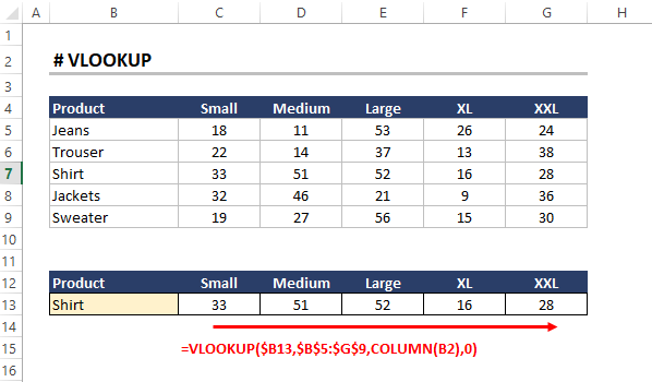
Let’s apply Vlookup here in the above Excel data of the cloth shop
He is looking for the product shirt and its available size in stock. In the above table, you will see different products listed in column B and their available sizes from Columns C to G.
Formula: =VLOOKUP($B13,$B$5:$G$9, Column(B2),0)
Lookup Value- Shirt
Table Array-B13 (Here we want to find our data) and B5 to G9 (The whole table where the data is searched )
col_index_num: Column B2
range_lookup: 0
$: Here $ is used to fix the value. Generally in Excel, if we want to fix the value of any cell then we used it
Result:
| Product | Small | Medium | Large | XL | XXL |
|---|---|---|---|---|---|
| Shirt | 33 | 51 | 52 | 16 | 28 |
This function of Excel will help him easily search for any data without any error and saves time.
Hope now it’s even clear to you how to use the advanced Vlookup function.
2. XLOOKUP() Function
Scenario:
Let us consider that you are running a kid’s cloth shop. Then How you are managing a record of the inventory of your cloth stuff?
I think you are keeping a record of all these data with any CMS Software. Nope, then what about doing it manually with Excel?
That’s Good but do you use advanced Excel formulas for managing all these tasks? No
Oh no……… it means you are investing a lot of time in this simple task.
Don’t worry it’s not too late. We have explained a function for you with a simple example that you can also apply to your data. Just go through this and learn.
As you manage a large record and you need data on large-size shirts. if you will do all these manually then it takes a lot of time to search for any specific products. Here in the example below, you can see a store manager is looking for data on large-size Shirts.
If he will manually find this quantity then it’s time-consuming. Then What is the alternative option for him? XLOOKUP function?
What is XLOOKUP() Function ?
The XLOOKUP function in Excel searches a range or array for a specified value and returns the associated value from another column. It can search both vertically and horizontally and perform exact (default), fuzzy (closest), or wildcard (partial) matching.
We will explain the use of match type later on while using the formula. First, we will see how this function works with an example.
Formula: XLOOKUP(lookup_value, lookup_array, return_array, [if_not_found], [match_mode], [search_mode])
- lookup_value: The value you want to find in the lookup_array.
- lookup_array: The range of cells that contains the values you want to search through.
- return_array: The range of cells from which you want to retrieve the result. This range should correspond to the same size as the lookup_array.
- if_not_found: Optional. The value to return if the lookup_value is not found. If omitted, Excel will return an #N/A error.
- match_mode: Optional. This parameter determines whether you want an exact match or the nearest match. Possible values are 0 (exact match), -1 (exact match or smaller), 1 (exact match or larger), or 2 (wildcard match). If omitted, it uses an exact match by default.
- search_mode: Optional. This parameter determines the search direction (1 for vertical, -1 for horizontal) when using an exact match or wildcard match. If omitted, Excel will use a vertical search by default.
How does XLOOKUP Function work and help the Store manager?
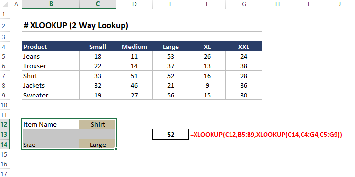
The Store manager needs the data on how many large-size shirts are left in the store
As you can see they have maintained a sheet where products are listed in column B and their different sizes from column C to G. Now the manager is interested to find a shirt(Product) of large size.
Let’s start working with XLOOKUP() function to get the result of the required query.
Formula: XLOOKUP(lookup_value, lookup_array, return_array, [if_not_found], [match_mode], [search_mode])
Let’s insert this formula into the data mentioned above in the table.
Formula: =XLOOKUP(C12, B5:B9, XLOOKUP(C14, C4:G4, C5:G9))
Lookup Value:Shirt (The product type that we want in our search result)
Lookup Array: B5 to B9 (Here the function search for our desired product result which is a shirt)
Return Array: C12( Here we want to find our data on the sheet of product shirt)
Again XLOOKUP is applied
Lookup Value: Large Size (The product size type that we want in our search result)
Lookup Array: C4 to G4 (Here the function search for our desired result which is a shirt size type that is Large)
Lookup Array:
Return Array: C14 ( Here we want to find our data on the sheet of product shirt size)
The other parameters that are mentioned above are optional. It means we can add them if we want or else we can avoid them.
Result:
| Item Name | Shirt | |
| Size | Large
|
The desired output is 52 large-size shirts quantity.
This function provides a two-way lookup which means both horizontal and vertical. It is more flexible than Vlookup and Hlookup. Thus it increases efficiency and productivity.
Is it clear to you? How XLOOKUP works. Hope so….
We always try to explain in simple words for our readers. Hope you found this helpful.
How XLOOKUP Better than VLOOKUP()
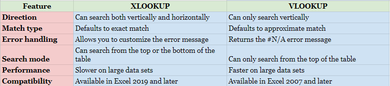
There are many more functions available in XLOOKUP in comparison to VLOOKUP. You can check below.
3. IF | IF OR | IF AND Function
Scenario:
When you are heading an accounts team of a big company and have to manage large records of data. Sometimes, maybe you feel it’s complex to manage the data accurately.
Rajesh working as an accounts Team Lead at a big MNC. Once, Rajesh has been instructed by the upper management to share a report on hikes of employee salaries of different departments.
Before that, he never manages such large data of employees who work in different departments at different locations. So he is a bit confused, about whether to calculate this one by one or to use the Excel function.
If Rajesh calculates this manually there is a chance of errors. Even it consumes a lot of time.
Rajesh finally decided to work fastly and submit the report on time. He already has an Excel sheet of different data as mentioned below in the example.
Now Rajesh uses the If function, and If OR functions to get the results as per the instructions.
Why he uses this function? It helps him to get the desired data quickly and with 100% accuracy.
What is IF() Function ?
The advanced IF function in Excel allows you to perform conditional evaluations and return different values based on a specified condition. It is widely used for logical and decision-making purposes in spreadsheets.
Formula: IF(logical_test, value_if_true, value_if_false)
- logical_test: This is the condition you want to check. It can be any logical expression that evaluates to either TRUE or FALSE.
- value_if_true: The value to be returned if the logical_test evaluates to TRUE.
- value_if_false: The value to be returned if the logical_test evaluates to FALSE
We will discuss first the IF function and then move to IF OR and IF AND with the same example.
How Does IF Function Works?
Let’s go through an example to understand how the IF function works and help Rajesh
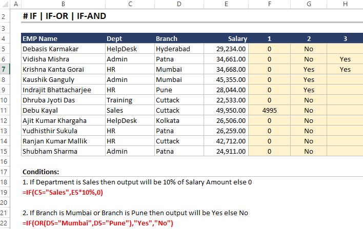
Here in the above example, you can see in the table, Employee’s name is mentioned in Column B. Their department is in Column C, Branch is in Column C, and salary data is in Column E.
Now here Rajesh wants to find if (the department is sales then the output will be 10% of the Salary Amount else 0)
Formula: =IF(C5=” sales”, E5*10%,0)
Logical Test: If the department is sales (C5= “sales”)
Value if True: Output will be 10% of the salary
Here, salary is mentioned in column E and for sales, its E5 so the output will be E5*10%
Value If False: If the department is not sales then return the value zero(0)
Result:
As you can see below the result is displayed in column 1. For sales, it displays a value of 4995 and for the rest, it’s showing 0.
Now, we will move toward the
IF-OR function
Formula: =IF(OR(condition1, condition2, …), value_if_true, value_if_false)
- condition1, condition2, etc.: These are the multiple conditions you want to check. They can be any logical expressions that evaluate to either TRUE or FALSE.
- value_if_true: The value to be returned if any of the specified conditions evaluate to TRUE.
- value_if_false: The value to be returned if all of the specified conditions evaluate as FALSE.
Now Rajesh wants to find if the branch is Mumbai or Branch is Pune then the output will be Yes else No
Formula: IF(OR(D5= ”Mumbai”, D5=” Pune”),” Yes”,” No”)
Here the branches are available in Column D
Condition 1: If the Branch is Mumbai (D5=Mumbai)
Condition 2: If the Branch is Pune (D5=Pune)
Value_if_True: Yes
Value_if_False: No
Result:
The desired result is mentioned above in the image as you can see.
The last one is
If And Function
Formula: IF(AND(condition1, condition2, …), value_if_true, value_if_false)
- condition1, condition2, etc.: These are the multiple conditions you want to check. They can be any logical expressions that evaluate to either TRUE or FALSE.
- value_if_true: The value to be returned if all of the specified conditions evaluate to TRUE.
- value_if_false:The value to be returned if any of the specified conditions evaluate to FALSE.
Let’s see this with an example, Rajesh’s Manager now asked him to share the salary data of employees.
But for that employee only whose salary is between 30000-35000.Rajesh can use if and function then easily he can get the required data.
If the Salary is between 30000 and 35000 then the output will be Yes else Blank cell
Formula: IF(AND(E5>=30000, E5<=35000)” YES”,” “)
Below is the image you can see in the third column that is representing this data
But if you are interested to learn all the functions with practical experience then you can join MS Offfice Course
4. SUMIF() Function
Scenario:
Have you read the previous scenario of Rajesh?
Just now he completed the previous task. But his manager doesn’t want Rajesh to seat without any work. Just joking……
Rajesh’s Manager has asked him to submit the annual salary report of different departments.
As Rajesh has an Excel Sheet, where he maintains all the data. But it seems too difficult for Rajesh to calculate manually without any mistakes.
Then he called his friend and asked to suggest an Excel Formula if he know that will help him to complete his task.
Rajesh’s friend advised him to use SUMIF Function. Want to know How? He use the SUMIF() function to do this task.
What is SUMIF() Function ?
The SUMIF() function in Excel is used to sum values based on a specified condition or criteria. It allows you to add up values that meet a specific requirement.
Formula: SUMIF(range, criteria, [sum_range])
Now, let’s break down the parameters:
- range: This is the range of cells you want to evaluate against the criteria. It is the range that will be checked for the condition.
- criteria: This is the condition that you want to apply to the cells in the range. It can be a number, text, expression, or cell reference.
- sum_range (optional): This is the range of cells that you want to sum up if their corresponding cells in the range meet the criteria. If not provided, the function will use the same range as the range parameter for the summation.
How Does SUMIF() Function Work?
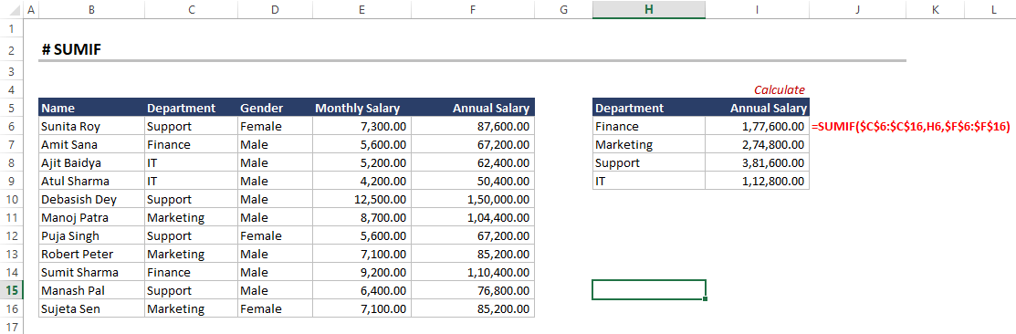
Now see how Rajesh uses this function to prepare the final report.
Let’s apply the function to the above data
Formula: =SUMIF($C$6: $C$16, H6, $F$6: $F$16)
Range: C6 to C16 ( Here he wants to apply the function against the mentioned Criteria)
Criteria: Finance, Marketing, Support, IT ( This is the criteria against which we want our sum data)
Sum_range: F6 TO F16 (This is the range of salary data (column F) that will be summed up in their corresponding cells in column C to meet the criteria)
Result:
| Department | Salary |
|---|---|
| Finance | 1,77,600.00 |
| Marketing | 2,74,800.00 |
| Support | 3,81,600.00 |
| IT | 1,12,800.00 |
5. OFFSET +SUM Function
Scenario:
Henry is running a bangles shop. Due to some health issues, the doctor advised him to take bed rest for at least 10 days.
He calculated that as per the suggestion, he can not go to the shop from (03.07.2023 – 13.07.2023).
After taking a rest, Henry is back to work and asked the Store Manager who is handling all his work in his absence. To show the data of total bangles sales quantity.
As the store manager knows well that Henry will ask for this data. So he keeps the data of all bangle’s date-wise sales quantity in an Excel sheet.
He knows OFFSET+SUM Functions also. Within a fraction of a second, he applied this function and share the data with Henry.
Henry thought the store manager will take time. But he submitted the details soon. In curiosity, Henry asked How you have done this.
Is there any Excel formula for this? The manager replied “Yes” OFFSET+SUM advanced Excel function
What is the OFFSET + SUM Function?
The OFFSET + SUM combination in Excel allows you to create a dynamic range and then sum the values within that range. The OFFSET function helps define a new range based on a starting point, and the SUM function then adds up the values within that new range. This combination is useful when you need to perform calculations on a changing range of cells.
- reference: This is the starting cell from which the new range will be defined.
- rows: This is the number of rows to move from the reference cell to determine the starting row of the new range. It can be a positive or negative value.
- cols: This is the number of columns to move from the reference cell to determine the starting column of the new range. It can be a positive or negative value.
- height (optional):This is the number of rows in the new range. If not specified, the new range will be one cell high.
- width (optional): This is the number of columns in the new range. If not specified, the new range will be one cell wide.
How Does OFFSET + SUM Function Work?
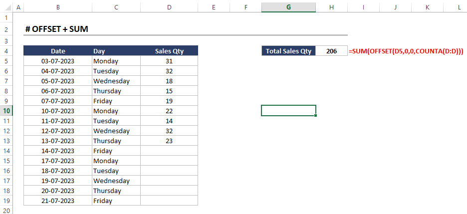
Formula: =SUM(OFFSET(D5,0,0, COUNTA(D:D)))
Reference: D5(This is the reference cell, which is the starting point for the new range.)
Rows: CountA(D:D) (This part of the formula calculates the number of rows to move up from the last cell in column D (13.07.2023) to reach the first cell of the new range (03.07.2023.)
The OFFSET function will create a new range representing the sales figures. After that SUM function sum up the sales values within the new range.
Once the store Manager applies this formula to the above data he will get the result of exact sales from 03.07.2023 to 13.07.2023
Result:
| Total Sales Quantity | 206 |
|---|
The next function in the Advance Excel Formula list is COUNTA(). Let’s dive into this with real-life scenarios.
6. COUNTA() Function
Scenario:
Let’s consider you are running a coaching center and a few days back you hired a center manager to manage all the teachers.
Once the center manager has joined the coaching, he wants to know the total no of teachers currently working.
Now as a center owner you handover him all the Excel records of the teacher’s data and told him to get the details from this.
The center manager started calculating the total no of teachers manually. One of his center teachers saw him calculating manually.
The staff teacher guided the center manager to use Advanced Excel Formula for these calculations.
See below How the teacher guided the center manager to use COUNTA() Function in the Excel sheet. Managers quickly get the results—the total no of a teacher working in the coaching institute.
As a manager, you can also learn Advance Excel Functions. Let’s start first with What is COUNTA Function and how the manager uses this function also.
What is COUNTA() Function ?
The COUNTA function in Excel Formula is used to count the number of cells in a range that are not empty. It includes both numerical values and text entries, making it useful for counting non-blank cells.
Formula: COUNTA(value1, [value2], …)
value1, value2, etc.: These are the arguments representing the cells or values you want to count. You can provide up to 255 arguments.
How Does COUNTA() Function Work?
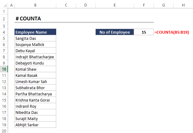
Just apply the above-mentioned formula
Formula: =CountA(B5:B19)
Result:
| No of Employee | 15 |
|---|
The COUNTA() function is particularly useful for data analysis tasks, where you need to determine the number of cells with data
Here you can see how a manager can easily calculate the staff number which is 15.
This advanced Excel formula makes it easy for the Manager to count staff no. Even the owner is also impressed.
7. COUNTIF() Function
Scenario:
Let’s walk through an example that you recently joined as an Assistant HR Executive in ABC Pvt. Ltd. Your manager assigned you a task to submit data on the total no of employees in each respective department.
Now You have two ways to calculate this
- Manually
- Use Excel Functions
To your knowledge, Which works best with maximum productivity and efficiency the answer is Excel Function.
Which Excel function you can use to prepare the report “COUNTIF() function”? But many are still not aware of this function and How to use it.
Don’t Worry! We are here to explain.
What is COUNTIF() Function ?
The COUNTIF() function in Excel is used to count the number of cells within a range that meet a specified criterion. It allows you to count cells based on specific conditions or criteria.
Formula: COUNTIF(range, criteria)
- Range: This is the range of cells you want to evaluate against the criteria. It is the range that will be checked for the condition.
- Criteria: This is the condition that you want to apply to the cells in the range. It can be a number, text, expression, or cell reference.
How Does COUNTIF Function Work?
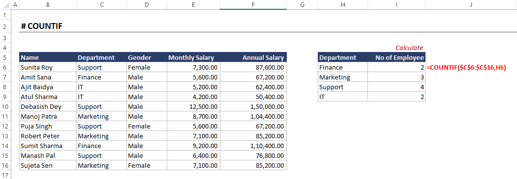
As you can see in the above image there is a complete employee details sheet.
Let’s start working with this sheet to get the total no of employees in different departments. Apply the formula
Formula: =COUNTIF($C$6:$C$16, H6)
Range: C6 to C16 ( Here we want our criteria to be checked)
Criteria: You have selected the different departments like Finance, Marketing, Support, and IT.
When you apply the formula to your data. The following result you get
Result:
| Department | No of Employee |
|---|---|
| Finance | 2 |
| Marketing | 3 |
| Support | 4 |
| IT | 2 |
Hope this information helps you to improve your Excel Knowledge.
8. MATCH() Function
Scenario:
Let us consider the case of the bank where you are working. The bank circulated a list of customers with their transaction IDs who came under the defaulter list in paying EMI.
The branch manager shared one Transaction ID with you and asked to share the position number of this ID in the Excel Sheet. With the help of the position number manager then analyze further details of EMI laps or issues.
The manager mentioned to you that he needs this urgently because there is some issue with that particular customer transaction.
As per your manager’s instructions, you need to submit this report soon. What are the options you have, either find it manually or use any smart strategy.
Yes, you can use advanced Excel Formula MATCH to find this. It will give you result quickly and without any error.
What is MATCH() Function ?
The MATCH() function in Excel allows you to find the position of a specified value within a range. It is commonly used in combination with other functions like INDEX() to perform advanced lookup and retrieval operations.
Formula: MATCH(lookup_value, lookup_array, [match_type])
- lookup_value:This is the value you want to find within the lookup_array.
- lookup_array:This is the range or array in which you want to search for the lookup_value.
- match_type (optional):This parameter specifies the type of matching to be performed. It can be one of the following values:
- 1 (or omitted): Finds the largest value less than or equal to the lookup_value (default).
- 0: Finds the first exact match to the lookup_value. The lookup_array must be sorted in ascending order.
- -1: Finds the smallest value greater than or equal to the lookup_value. The lookup_array must be sorted in descending order.
How Does the MATCH() Function Works?
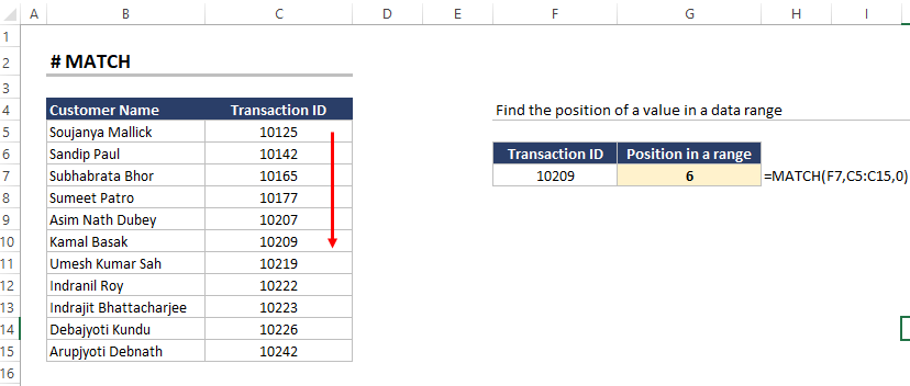
When you apply the formula in your data sheet you can easily find the result. Check below how it will help you.
Formula: MATCH(F7, C5:C15,0)
Lookup Value: 10209 (This is the value we want to find in the lookup_array)
Lookup Array: C5:C15 (This is the range or array in which we want to search for “10209.”)
Match Type: 0 (The match_type is set to 0 to find the first exact match)
After applying the formula see how easily you can get the result
Result:
| Transition ID | Range |
|---|---|
| 10209 | 6 |
9.INDEX+ MATCH /VLOOKUP + CHOOSE Function
Scenario:
Have you read the previous case? If so then let’s move with that only with one more query.Yes, Now your manager wants to send a notice to that customer who is not paying EMIs for the last three months.
In this regard, your manager asked you to share the customer name of that transaction ID that he shared with you.
Don’t worry, if you have no idea how to find this quickly.We will explain to you the quick process to get this result.
There are two different ways you can use to get this result, which means two different Excel functions
-
- INDEX+ MATCH Function
- VLOOKUP + CHOOSE Function
What is the INDEX+ MATCH Function ?
The combination of INDEX and MATCH functions in Excel is a powerful way to look up and retrieve specific data from a table.
The INDEX function returns the value of a cell in a specified row and column within a range. While the MATCH function is used to find the position of a lookup value within a given range.
When used together, they allow you to perform a two-dimensional lookup, where you can find a value based on both row and column criteria.
Formula (INDEX Function): INDEX(array, row_num, [column_num])
Formula (MATCH Function): MATCH(lookup_value, lookup_array, [match_type])
- array:This is the range or array from which you want to retrieve the data.
- row_num:This is the row number from which you want to get the value.
- column_num(optional): This is the column number from which you want to get the value. If omitted, the function returns the value from the specified row only.
- lookup_value: This is the value you want to find within the lookup_array.
- lookup_array: This is the range or array in which you want to search for the lookup_value.
- match_type (optional):This parameter specifies the type of matching to be performed
How Does the INDEX + MATCH Function Work?
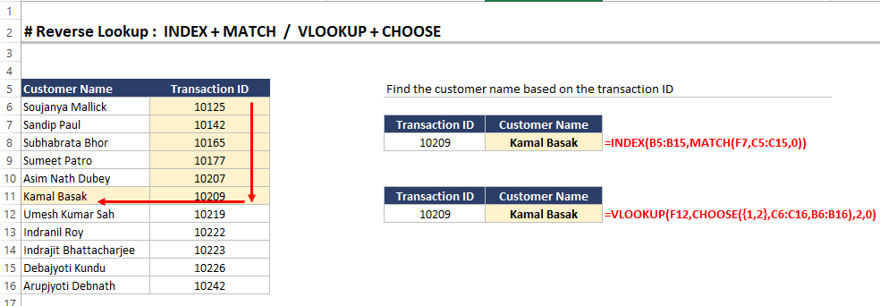
Formula(INDEX + MATCH): INDEX(B5:B15, MATCH(F7, C5:C15,0))
Array: B5:B15 (This is the array from which you want to retrieve the data).
Row_num: F7 (This is the row number (Customer ID) you want from the MATCH function.)
Lookup Value: Customer Name (The name of the customer you want as per the Transition ID)
Lookup Array: C5:C15 (This is the range or array in which you want to search for the customer name).
Match Type :0
After successfully applying the formula your result will be there in a fraction of a second.
Result:
| Transaction ID | Customer Name |
|---|---|
| 10209 | Kamal Basak |
This is the first way to find the required details. Let’s see another option in detail
VLOOKUP + CHOOSE Function
What is VLOOKUP + CHOOSE Function
The combination of VLOOKUP and CHOOSE functions in Excel allows you to perform more complex lookups and get data from different columns based on a single criterion.
The VLOOKUP function looks for a value in the leftmost column of a range and returns a corresponding value from a specified column within that range.
The CHOOSE function allows you to select a value from a list of values based on a numeric index. When used together, you can dynamically choose which column to look up the data based on the result of another function.
Formula (VLOOKUP): VLOOKUP(lookup_value, table_array, col_index_num, [range_lookup])
Formula ( CHOOSE): CHOOSE(index_num, value1, [value2], …)
- lookup_value: This is the value you want to find in the leftmost column of the table_array.
- table_array: This is the range or array containing the data to be searched. The lookup_value should be in the leftmost column of this range.
- col_index_num:This is the column number within the table_array from which the result should be returned.
- range_lookup (optional):This parameter is either TRUE (approximate match) or FALSE (exact match). If omitted, it defaults to TRUE.
- index_num: This is the numeric index that specifies which value to select from the list of values provided in the CHOOSE function.
- value1, value2, etc.:These are the values from which you want to choose based on the index_num.
Now, we will see how this function helps you.
How Does the VLOOKUP + CHOOSE Function Work?
Formula: VLOOKUP(F12, CHOOSE({1,2}, C6:C16, B6:B16),2,0)
Lookup Value: Customer Name
Table Array: B6 to B16
Col_index_num: F12
Index_num:
The following result will be displayed
Result:
| Transaction ID | Customer Name |
|---|---|
| 10209 | Kamal Basak |
This combined function helps you to perform lookups based on different criteria. Then you can choose which data you want.
If you are still confused about how these different Excel functions work in different cases. You can check the courses on MS Office that are designed by ICA experts.
For sure it will help you to clear the basic concepts of advanced Excel functions and formulas.
10. CONCATENATE() Function
Scenario:
A coaching center manager is organizing a guest lecture for students. For the same, he is writing the name of students who are interested to join that guest lecture.
He started writing the name of students in Excel with the first name in one column and the last name in one column. Once he completed the enrollment of the student.
The Center owner asked the manager to submit the list. But he mentioned that write the full name in one column.
But the manager has written it in two different columns. So, he is worried that he have to write it again.
Do you have any idea about any Excel function which can complete the task of manager in a short time?
No, We will tell you How you can do this. It’s so simple just use the CONCATENATE function in Excel.
What is CONCATENATE Function ?
The CONCATENATE function in Excel is used to combine multiple text strings into a single string. It allows you to join together the contents of two or more cells or add additional text or characters in between the cell values
Formula: CONCATENATE(text1, [text2], …)
text1, text2, etc.:These are the text strings or cell references that you want to concatenate. You can include up to 255 text strings or cell references.
How Does the CONCATENATE Function Work?
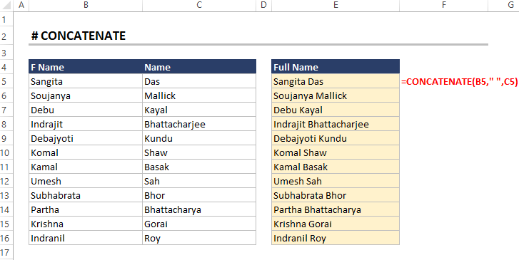
Formula: =CONCATENATE(B5, “ “, C5)
After applying the formula to the student name list. You can get the result like this:
Result:
| Full Name |
|---|
| Sangita Das |
| Soujanya Mallick |
| Debu Kayal |
| Indrajit Bhattacharjee |
| Debajyoti Kundu |
| Komal Shaw |
| Kamal Basak |
| Umesh Sah |
| Subhabrata Bhor |
| Partha Bhattacharya |
| Krishna Gorai |
| Indrani Roy |
11. REPT Function
Scenario:
Let’s move with the same previous example. Now the owner asked the students to give a rating to this guest lecture from 1 to 5. Students have shared the details with the center manager.
But the center owner advised the manager to add a string of rating stars in one column of the Excel sheet. So that it looks perfect when he will share this with the center director.
Now, the manager has to add * as a string with the respective rating number.
As per instructions if the manager wrote * manually after each rating no in the next column. Then, it’s too time-consuming matter.
But he is smart because he uses the REPT function to prepare this data.
What is REPT Function ?
The REPT() function in Excel allows you to repeat a text string a specified number of times. It is useful for creating repeated patterns or generating repetitive text values.
Formula: =REPT(text, number_times)
- text: The text string that you want to repeat.
- number_times: The number of times that you want to repeat the text string.
How Does the REPT Function Work?
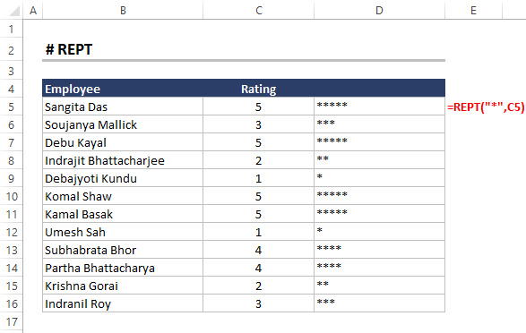
Formula: =Rept(“*”, C5)
Text: * (This string is inserted repetitively).
Number_times: Number of times we want * to be repeated in the sheet.
Result:
In the above image, you can see that * is written as the no of times a numerical value is given to it.
12.TYPE FUNCTION
Scenario:
Let’s consider that a session is organized for 8 class students on MS Excel. One task given to all the students was to differentiate the data mentioned on the Excel sheet based on a numerical value
The teacher has given students the Excel sheet and the information on the numerical value according to the data type
As per the instruction by the teacher, the student started preparing the sheet. In the beginning, all students are doing it manually.
Students are checking the pre-given information that if data is a number then write 1. If the data is text then write 2.
Later on, when students did not submit the task on time. The teacher has taught them the TYPE function to complete the assignment.
What is the TYPE Function ?
The TYPE() function in Excel allows you to determine the type of data contained within a cell. It returns a numerical code that corresponds to a specific data type. This function is useful when you need to identify the type of data stored in a cell or a formula result.
Formula: =TYPE(value)
- value: The cell reference or the value that you want to determine the type of.
The TYPE function returns the following numerical codes for different data types:
- 1: Number
- 2: Text
- 4: Logical (Boolean)
- 16: Error
- 64: Array
- 128: Cell reference
How Does the TYPE Function Work?
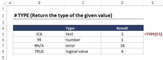
Formula: =TYPE(C5)
When the formula is applied to the above data, it represents the numerical value according to the type of inserted data.
For example, For the text ICA it shows the value of 2 because ICA comes under the text category.
Result:
You can see in the above image how easily one can determine the type of data value with the help of the Type function.
13.LEFT_MID_RIGHT Function
Scenario:
Let’s start with the simple example of a grocery store that deals with multiple products and operating in multiple states. The account manager is maintaining an EXCEL sheet, where he is writing the GSTINs of each operating state.
Once the store owner asked to share the report of each state GSTINs details with state code, PAN, and the last three digits in three separate columns. So that it will be easy for him to understand
The account manager is maintaining a sheet so it will be easy for him to get this result. But he doesn’t want to do this manually because it consumes a lot of time.
He has an idea about the LEFT, MID, and RIGHT functions that will easily do this.
Let’s explore how the account manager uses this feature of Excel to prepare the report.
What is LEFT_MID_RIGHT Function ?
The LEFT, MID, and RIGHT functions in Excel are used to extract parts of a text string. The LEFT function extracts the first n characters from a text string, the MID function extracts a specified number of characters from a text string starting at a specified position, and the RIGHT function extracts the last n characters from a text string.
The LEFT, MID, and RIGHT functions are all very similar, but they have some key differences.
The LEFT function always extracts the first n characters from a text string, regardless of where the nth character is located.
The MID function extracts a specified number of characters from a text string starting at a specified position. The position can be specified as an absolute position or as a relative position.
The RIGHT function extracts the last n characters from a text string.
How Does the LEFT_MID_RIGHT Function Work?
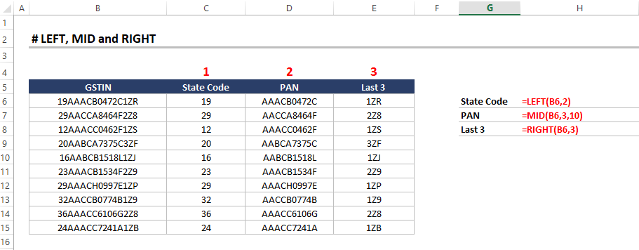
Let’s apply these three functions in the above image of the datasheet of guest list details
We will apply all the formulas in column B where GSTIN (Unique ID List created by the hotel) is written.
So, When we apply the LEFT function it displays the result as START CODE
= LEFT(B6,2)
Here we have selected the complete B column starting from 6, and the first two digit number it displays from the text string
After that apply the function MID
=MID(B6,3,10)
Here we have selected Column B and from this, it selects from 3 characters to 10 characters from the text string.
The last one is the RIGHT Function
=RIGHT(B6,3)
Here we have selected Column B and the last 3 characters will display
Results:
You can see the result of all three functions in the above image as Start Code, PAN, and Last 3.
Whenever you find this type of data problem to solve, you can use advanced Excel functions for analysis. It’s easy to implement these functions and get quick results in a short period.
It increases your work efficiency and productivity.
You can explore here more about Advance Excel Courses
14. RANDBETWEEN() Function
Scenario:
Let’s imagine you are the marketing manager of an e-commerce store. To increase sales you have decided to run a promotional campaign to attract more customers.
The goal you have set is to offer random discounts to customers as an offer to attract them for purchasing your products.
According to your goal, You are offering 5% to 20% of discount on their total purchase amount.
Now you have to create the sheet where you will add discounts for customers. If you will prepare the discount sheet manually for customers it takes a lot of your time.
So, How you will manage this situation?
You can use the RANDBETWEEN() function in Excel to generate random discount values within 5% to 20%. Based on the percentage discount then you can calculate the discounted amount on their total bill.
What is RANDBETWEEN Function ?
The RANDBETWEEN function in Excel generates a random number between two numbers that you specify.
Formula: RANDBETWEEN(lower_bound, upper_bound)
- lower_bound: The smallest number that the function can return.
- upper_bound: The largest number that the function can return.
The RANDBETWEEN function will always return a number that is greater than or equal to the lower_bound and less than or equal to the upper_bound
How Does the RANDBETWEEN Function Work?
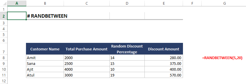
Formula: =RANDBETWEEN(5,20)
Let’s apply this formula in the above datasheet.
Lower Bound: 5% ( It means the minimum discount that can be given to customers is 5% on their purchase)
Upper Bound: 20%(It means the maximum discount that can be given to customers is 20% on their purchase)
In cell D2 (the first row under “Random Discount Percentage”), enter the formula =RANDBETWEEN(5, 20). This will generate a random whole number between 5 and 20 as the discount percentage for the first customer.
To calculate the discounted amount for each customer, use the formula =[@’Total Purchase Amount’] * (1 – [@’Random Discount Percentage’]/100) in cell D2 (the first row under “Discounted Amount”). This formula will calculate the discounted amount based on the respective customer’s total purchase amount and random discount percentage.
Result:
You can see in the above image that after applying the formula random discount for each customer is generated. After that discounted amount is calculated. All the discount percentages are between 5 to 20.
15. CONVERT
Scenario:
The school teacher is taking an Excel class and gives the students one task to convert the product weight data mentioned from Kg to gram.
The list of products is too many and the teacher gives the time of 15 mins to complete this task
There are few students who know how to complete this on time by using the CONVERT Function of Excel. But there are many students who started doing manual calculations.
After knowing this situation teacher started explaining the advanced Excel formula CONVERT to get the results.
Let’s see how the teacher explains this formula
What is CONVERT Function?
The CONVERT() function in Excel is a powerful tool for unit conversion. It allows you to convert a value from one measurement unit to another.
Formula: =CONVERT(number, from_base, to_base)
- number: >The number that you want to convert.
- from_base: The base of the number that you want to convert from.
- to_base: The base of the number that you want to convert to.
How Does the CONVERT Function Work?
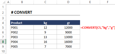
Formula: =CONVERT(C5,” kg”,g”)
Number: C5 (The kg column that we want to convert)
From_base: Kg(The base of the number that we want to convert from).
To_base g(The base of the number that we want to convert to).
When we apply the above formula it will convert all the measurements from Kilogram(kg) to gram(g).
Result:
You can see in the above image where the final data on converted product weight is written in gram(g)
Hopefully you have also got an idea of each advanced Excel formula with examples that we have explained till now.
16. SUMPRODUCT() Function
Scenario:
Let’s see an example that you are running a books shop. For each day of sales of the most expensive book in your store, you are maintaining a sheet with product quantity sold with their prize.
You are maintaining a sheet for the whole week means from Monday to Saturday. You have created day-wise so that you can check the data each day wise. Also if needed to calculate the total sales of the most expensive item of the whole week.
Now on Sunday, you are calculating the final total sales of the books. But have no idea how to do this quickly instead of one by one.
You searched on Google and Google answered you to use SUMPRODUCT function.
What is SUMPRODUCT Function?
The SUMPRODUCT() function in Excel is a versatile tool for performing calculations on arrays or ranges. It allows you to multiply corresponding values in multiple arrays or ranges and then sum the products.
Function: =SUMPRODUCT(array1, array2, …)
- array1: The first array.
- array2: The second array.
- …: Additional arrays.
How Does the SUMPRODUCT Function Work?
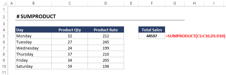
Formula: =SUMPRODUCT(C5:C10, D5:D10)
- array1: C5: C10 (The first array of data that we want to multiply)
- array2: D5:D10 The second array of data from which the first array is multiplied)
After that final result is the sum of all the multiplied values.
For Example C5* D5 + C6*D6 + ……
Result:
| Total Sales |
|---|
| 44597 |
See, it’s so easy. We hope now you can do this type of calculation by using the SUMPRODUCT formula.
17. IFERROR() Function
Scenario:
Sneha works in a Cosmetic shop as sales Person. The cosmetic shop owner once asked Sneha to share a report on the average sales price of all products.
The owner also suggested to Sneha that if there is any product in the stock whose sales are 0. Then also mention that in the sheet and give a 0 value to that product in the list.
Sneha has not prepared that large data sheet previously. So she has no idea how to prepare this without any mistakes and quickly.
We will explain how she can simplify this work with IFERROR Function
What is IFERROR Function?
The IFERROR() function in Excel allows you to handle and manage errors in formulas. It helps you control the output or display a specific value when an error occurs. In simple words
The IFERROR function in Excel returns a value you specify if a formula evaluates to an error; otherwise, it returns the result of the formula
Formula: =IFERROR(formula, value_if_error)
- formula: The formula that you want to check for errors.
- value_if_error:The value that you want to return if the formula evaluates to an error.
How Does the IFERROR Function Work?
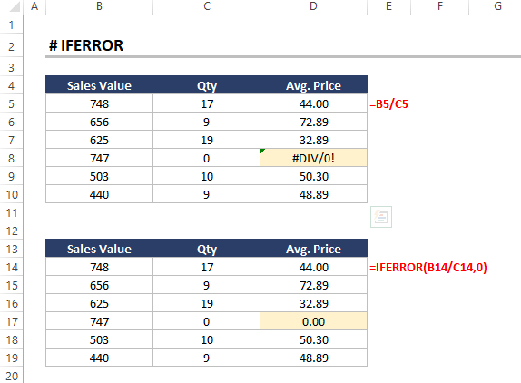
Sneha can first create the sheet of average prices and then she can apply the IFERROR formula.
Formula = IFERROR(B14/C14,0)
Let’s evaluate the Excel data sheet with the IFERROR function.
In the above image of the first datasheet, as you can see, the average value(Avg Price) is calculated by dividing the total sales by the total quantity(B5/C5).
In the second datasheet of the same image when we apply the IFERROR function then it evaluates. if the average price is B14/C14 then the value is written else and displays 0 as an error.
Result:
In the above image you can check the result of the applied function
Key Takeaways:
If you are fed up with manual work and want to use advanced Excel formulas. So you are in a good place.
You can learn complete advanced Excel formulas from the experts.

Looking for knowledge booster articles read here
Top 10 Techniques | Microsoft Advanced Excel Certifications
2022 Apply For Most Demanding Advanced Excel Courses
All-Purpose Benefits Of Microsoft Office Specialist Certification Courses
We have tried to cover all the important Excel formulas widely used by data scientists. For ease of understanding, we have used real-life examples to help you clarify your basic concepts.
These days the demands of Advanced MS Excel experts are high as most companies now completely rely on data for their better business workflow. They always look for experts in this field and if you become then it’s easy for you to grab a big opportunity in your career.
Check Out Frequently Asked Advanced Excel Interview Questions
1.What is the difference between VLOOKUP and HLOOKUP?
VLOOKUP searches for a value in the first column of a range and returns the value in the same row from a specified column. HLOOKUP searches for a value in the first row of a range and returns the value in the same column from a specified row.
2.What is the purpose of the MATCH function?
The MATCH function returns the position of a value in a range, starting from 1.
3.What is the INDEX function?
The INDEX function returns the value of a cell at a specified row and column.
4.What is the purpose of the OFFSET function?
The OFFSET function returns a reference to a cell that is offset from a specified cell by a specified number of rows and columns.
5.How the SUMPRODUCT function works in Excel?
The SUMPRODUCT function returns the sum of the products of corresponding values in two arrays.
6.How does the COUNTIF function help in Excel?
The COUNTIF function counts the number of cells in a range that contain a specified value.
7.Do you know about the COUNTA function?
The COUNTA function counts the number of cells in a range that are not empty.
8.What is the purpose of the IF function?
The IF function returns one value if a condition is true and another value if the condition is false.
9.Explain the VLOOKUP function in short?
The VLOOKUP function searches for a value in a table and returns the corresponding value from another column in the table.
10.What is the HLOOKUP function?
The HLOOKUP function searches for a value in a table and returns the corresponding value from another row in the table.
Explore more interview questions

Certification: Certified Microsoft Excel Expert and Tally, .
Profession: Ms Excel, TallyPrime Trainer
Organization: Corporate Trainer – Technical Quality Assurance at “ICA Edu Skills Pvt. Ltd".
Industry Experience - Expert of MS Office, Tally, VBA, SQL, Power BI with over 16+ years of experience, trained more than 7,000+ individuals and Delivered Master Classes for over 100+ trainers of Excel and Tally.
Linkedin Profile: https://in.linkedin.com/in/debjit-chakraborty-873b6887
- Purchase Order in Tally Prime: Manage Inventory & Expenses - June 7, 2024
- Payroll in Tally Prime: Process, Flow Chart, Features - April 26, 2024
- How to Create a Debit Note in Tally Prime - March 22, 2024